Cellular Automata, an intelligent technique for modeling complex systems

Andrés Julián Arias-Moreno
Full Time Professor
Bioengineering and Chemical Engineering Department

Artificial intelligence techniques have been around for several decades, and are not just limited to machine learning, neural networks, fuzzy logic or deep learning. There is a technique that allows modelling temporal states of highly complex systems and is able to predict changes in these systems by applying simple evolutionary rules. This artificial intelligence technique is known as the Cellular Automata paradigm.

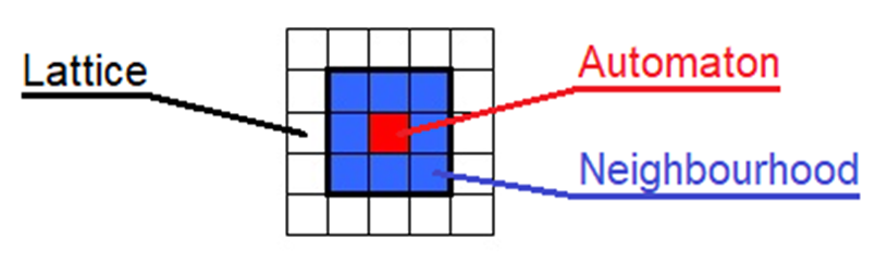
Cellular Automata (CA) are small elements that occupy spaces or unit cells within a discrete two- or three-dimensional domain called a lattice or grid, which volume represents the modelled system (Figure 1). Each automaton located in a cell of this lattice has a state, within a group of predefined states, which through interaction with itself and with its neighbouring cells can maintain or change through the iterations of evolution of the modelled system, because each automaton has the ability to make decisions independently to maintain or change that state as the system evolves. By projecting this automaton behaviour on a larger scale, it is possible to model highly complex systems whose macro behaviour is governed by the behaviour of its smaller component units.

**Figure 1. Configuration of a cellular automaton in its cell in a two-dimensional lattice [1].**

The evolution of the automaton’s state is based on the application of very simple individual evolution rules. In each iteration, the automaton knows only its own state and the state of its nearest neighbours, and depending on these states and the evolution rules, the automaton evolves to the next iteration either maintaining or changing its state.

The cells containing the automata, which in turn form the lattice or domain of the modelled system, may be square, triangular or polygonal in the two-dimensional case, or hexahedral or tetrahedral in the three-dimensional domain.

In order to know the state of its neighbours, the automaton uses a type of neighbourhood to relate to its environment, which depends on the number of neighbouring automata taken into account. The used neighbourhoods range from the empty neighbourhood, in which the automaton only takes itself into account, to the neighbourhoods that take into account four (von Neumann), eight (Moore), twelve (expanded von Neumann, MvonN) or twenty-four (expanded Moore) neighbours. The latter includes the neighbouring automata at the first and second level of distance (Figure 2, top).

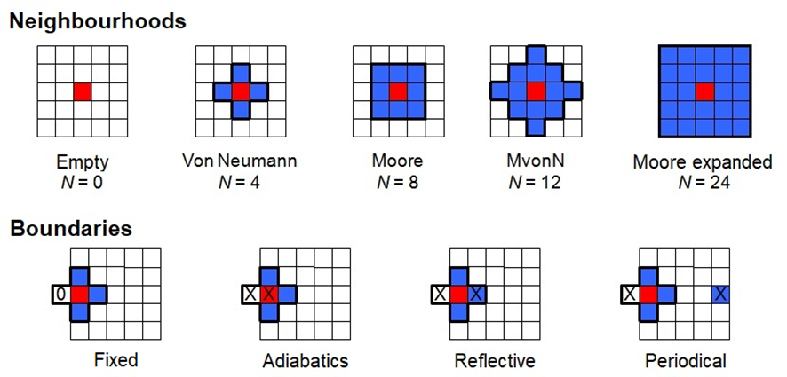
**Figure 2. Neighbourhoods (top) and Boundaries (bottom) considered in the implementation of cellular automata [2].**

When the automaton is at a boundary of the domain, it also takes into account different configurations for the hypothetical neighbouring cells located outside the boundary, which assign them specific states for iteration and evolution. Within the configurations for these out-of-domain positions, they can be assigned a null state (fixed boundary), the same state as the automaton on the boundary (adiabatic boundary), the same state as the automaton on the contralateral side of the boundary (reflexive boundary) or the state of the automaton on the same row at the opposite end of the lattice (periodic boundary), (Figure 2, bottom).

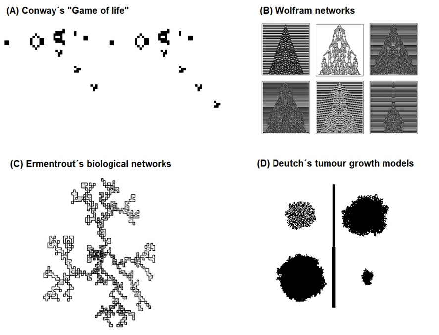
The cellular automata paradigm appeared in the 1940s by Stanislaw Ulam to describe graphically the growth of crystals. Simultaneously, Von Neumann used the same tool to study systems capable of self-replication. In the 1970s, John Conway used the concept of CAs to create the game of life, a model of the dynamic ability of automata to move and replicate themselves by implementing simple evolutionary rules (Figure 3, A). In 1983, Wolfram presents in his work a new kind of science the development of several rules that generate series of self-replicating regular and irregular shapes (Figure 3, B). In 1993, Ermentrout et al. used CAs for the first time in the generation of biological networks such as the neural system and the circulatory system, taking the model as a continuous process (Figure 3, C). By 2004, Deutch et al. developed the first models of tumour growth (Figure 3, D).

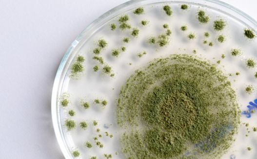
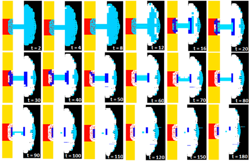
Figure 3. Historical developments of cellular automata: (A) Conway’s game of life, (B) Wolfram’s regular and irregular networks, (C) Ermentrout’s neural and cardiovascular networks, and (D) Deutch’s tumour growth models [1].

To date, cellular automata have been used to simulate and predict behaviour in diverse systems such as fractal formation, the behaviour of bacterial populations, traffic analysis in large cities, the creation of structures by topological optimisation, and even tissue architecture and healing time in a bone fracture repair process (Figure 4).

Figure 4. Two-dimensional axisymmetric model of cellular automata for the simulation of the process of osteogenesis and bone fracture repair. The architecture of the component tissues of the bone callus are represented with different colours (red: bone marrow; yellow: fatty bone marrow; light blue: granular and fibrous tissue; dark blue: cartilage; white: bone). The repair time t is given in days [1].

In summary, cellular automata, a prominent technique in artificial intelligence, allow the behaviour of a variety of highly complex systems to be analysed and predicted in a simple and straightforward manner.

References

[1] A.J. Arias-Moreno. “Modelo computacional para la simulación del proceso de osteogénesis y curación ósea después de la fractura”. Master thesis, Universidad Nacional de Colombia, Colombia, january 2011.

[2] A. Tovar. “Bone remodeling as a hybrid cellular automaton optimization process”. Doctoral thesis, University of Notre Dame, United States, december 2004.