Andrei Markov was a Russian mathematician who worked and contributed to the theory of stochastic processes. Markov strings describe a random process in which the future state of the system depends solely on its present state and not on its past history. Markov chains have numerous applications in fields such as physics, biology, chemistry, economics, computer science, engineering, etc.

Markov chains provide a powerful framework for modeling stochastic biological systems and have applications in genetics, bioinformatics, epidemiology, neuroscience. For example:

• In population genetics, Markov chains are used to model the genetic deviation that occurs when populations experience random fluctuations in allele frequencies;
• In bioinformatics, they are used to align multiple sequences and identify patterns of regions conserved in DNA or protein sequences;
• In Epidemiology: Markov models can be used to model the spread of infectious diseases where susceptible-infected-recovered (CRS) models are built that have states where people move between: susceptible, infected and recovered.
• In Neuroscience: Markov chains are used to model neuron activation patterns in response to stimuli or neural network connectivity patterns.

Markov strings are probabilistic graphical models that represent a dynamic process that changes over time. For any process to be considered for modeling with the Markov Chain, it must assume the Markov Property which states that the next state (t+1) depends only on the current state (t) and is independent of all previous states since (t-1, t-2, …), that is, to know a future state, we just need to know the current state.

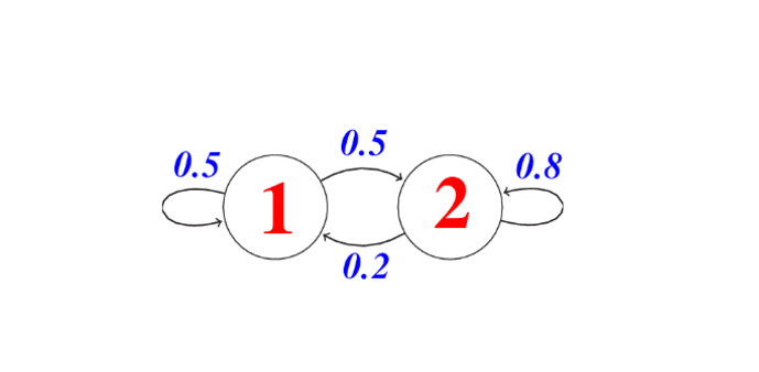
Then we can see a Markov chain (MC) as a discrete state machine with nondeterministic transitions between states, that is, there is a probability of transiting from one state “p” to another state “k”. Formally, a Markov string of n states and having S0 as the initial state is specified with the following three elements:

• Set of states: Q = {S1, S2, . . . , Sn}
• Probabilities of occurrence of each state: Π = {π1, π2, . . . , πn}, where πk = P(S0 = qk)
• State change probabilities: P(St = K | St 1 = p )

A Markov string model can help answer basically three types of questions:

• What is the probability of a given sequence of states?
• What is the probability that the chain will remain in a certain state for a period of time?
• What is the expected time the chain will remain in a given state?

Estimating parameters of a Markov chain remains a challenge. For some models, parameters can be estimated by simply counting the number of times the sequence is in a certain state, p, and the number of times there is a transition from a state p to a state k. If we have N sequences of observations. λ0p is the number of times the p-state is the initial state of a sequence, λp is the number of times we observe the state p and λpk is the number of times we observe a transition from the state p to the state k. The initial probabilities would be πp = λ0p/N and the transition probabilities would be apk = λpk/λp

Markov hidden strings (HMM) are used when states cannot be directly observed, but only the result of some state probability function. HMM is a statistical model in which the system being modeled is supposed to be a Markov process with unobserved (hidden) states. A Markov model is useful when we need to calculate a probability for a sequence of observable events. However, in many cases the events that interest us are not directly observed. An HMM allows us to talk about observed events and occult events that we consider as causal factors in our probabilistic model.

An example would be the recognition problem of the 5′ splice site of a DNA (Fig 3). If you give us a DNA sequence that starts in an exon, it contains a 5′ splice site and ends in an intron. The problem is to identify where the switch from exon to intron occurred, where the 5 (5 SS) splice site is. If the exons have a uniform base composition on average (25%), the introns are rich in A/T (40% each for A/T, 10% each for C/G) and the 5’SS consensus nucleotide is almost always a G (95% G and 5% A).

With this information we can draw an HMM (Fig. 3) that has three states, one for each of the three labels that we could assign to a nucleotide: E (exon), 5 (5 SS) and I (intron). Each state has its own emission probabilities, which model the base composition of exons, introns and the G consensus in the 5 SS. Each state also has transition probabilities (arrows), the probabilities of passing from this state to a new state. The model generates two chains of information if when visiting a state, a residue of the probability distribution of emission of the state is emitted and then another state goes according to the transition probability distribution of the state. The first represents the state path (tags) as we transition from one state to another and the second represents the observed sequence (DNA). The state path is a Markov string because the next state depends only on the present state. Since only the observed sequence is given, this state path is hidden and are the waste labels used. The state road is a hidden Markov chain. Finally, the probability P(S,π|HMM,θ) that an HMM with θ parameters generates a state path π and an observed sequence S is the product of all the emission and transition probabilities that were used.

Although the problem of estimating an unknown discrete distribution from their samples was a complex problem and during the last decade a significant research effort was made that solved it for a variety of divergence measures. However, building and estimating an unknown Markov chain and its parameters from its samples is still a very complex problem.

Currently professors of Bioengineering at UTEC are working on projects related to Markov chains with biological applications. If you are interested in being part of the projects you expect: Join UTEC Bioengineering!

References:

1. Caswell, H 2001 Matrix Population Models. 2nd Ed. Sinauer Assoc. Inc., Sunderland, MA
2. Grassly NC, Fraser C. Mathematical models of infectious disease transmission. Nat Rev Microbiol. 2008;6(6):477–487.
3. Balzter H . Markov chain models for vegetation dynamics. Ecological Modelling. 2000;126(2–3):139–154.
4. Choo KH, Tong JC, Zhang L. Recent applications of Hidden Markov Models in computational biology. Genomics Proteomics Bioinformatics. 2004;2(2):84–96.
5. Koski T. Hidden markov models for bioinformatics. Springer Netherlands; 2001.
6. Eddy, S. What is a hidden Markov model?. Nat Biotechnol 22, 1315–1316 (2004). https://doi.org/10.1038/nbt1004-1315
7. Grewal, J.K., Krzywinski, M. & Altman, N. Markov models—Markov chains. Nat Methods 16, 663–664 (2019). https://doi.org/10.1038/s41592-019-0476-x
8. Djordjevic IB. Markov Chain-Like Quantum Biological Modeling of Mutations, Aging, and Evolution. Life (Basel). 2015 Aug 24;5(3):1518-38. doi: 10.3390/life5031518. PMID: 26305258; PMCID: PMC4598651.
9. Athey, T.L., Tward, D.J., Mueller, U. et al. Hidden Markov modeling for maximum probability neuron reconstruction. Commun Biol 5, 388 (2022). https://doi.org/10.1038/s42003-022-03320-0
10. Chen, Y., Baños, R. & Buceta, J. A Markovian Approach towards Bacterial Size Control and Homeostasis in Anomalous Growth Processes. Sci Rep 8, 9612 (2018). https://doi.org/10.1038/s41598-018-27748-9
11. Armond, J., Saha, K., Rana, A. et al. A stochastic model dissects cell states in biological transition processes. Sci Rep 4, 3692 (2014). https://doi.org/10.1038/srep03692
12. Barra, M., Dahl, F.A., Vetvik, K.G. et al. A Markov chain method for counting and modelling migraine attacks. Sci Rep 10, 3631 (2020). https://doi.org/10.1038/s41598-020-60505-5

More posts